1D Example
Introduction
Regression problems typically involve estimating some unknown function \(f\) from a set of noisy data \(y\). As an example we can attempt to estimate a function \(f(x)\),
based off of noisy observations,
For this example we’ll use the sinc function for the non linear portion,
Model Definition
For illustrative purposes we’ll assume we know nothing about the non linear component other than that we think it’s smooth. To capture this with a Gaussian process we can use the popular squared exponential covariance function which states that the function value at two points \(x\) and \(x'\) will be similar if the points are close and less similar the further apart they get. More specifically the covariance between values separated by a distance \(d = |x - x'|\) will be given by,
Our first iteration may then say that the covariance between any two locations can be defined by
or in other words we’re saying our data comes from a smooth function and has some measurement noise where the measurement noise is given by,
and \(\mathbf{I}(b)\) evaluates to one if \(b\) is true and zero otherwise.
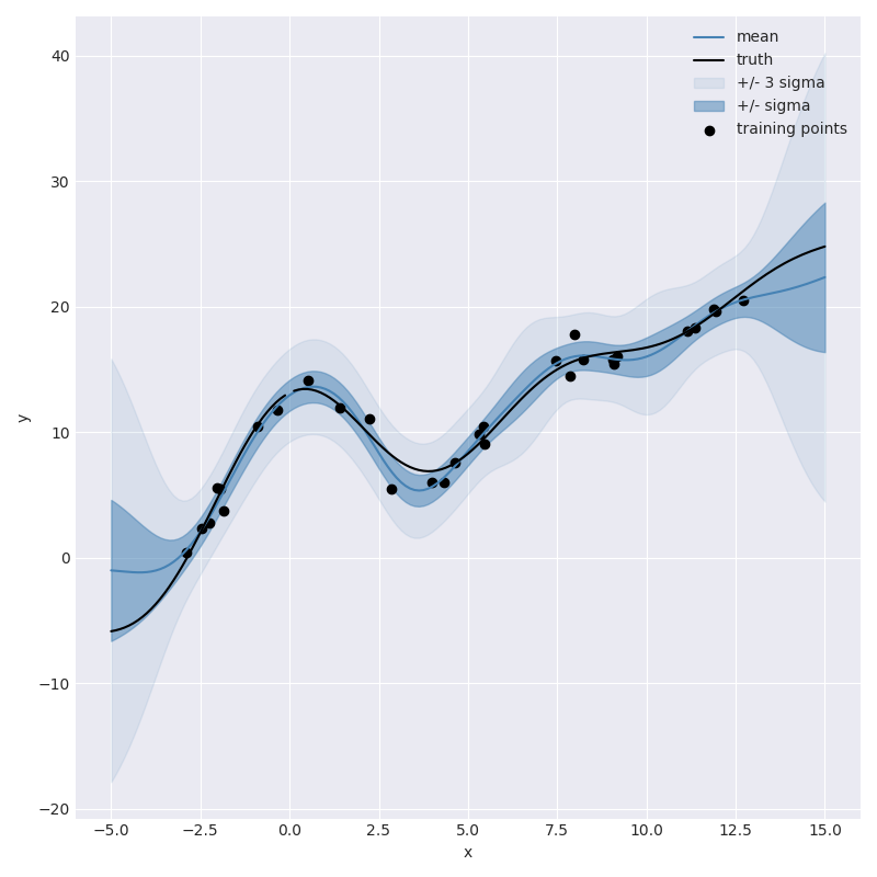
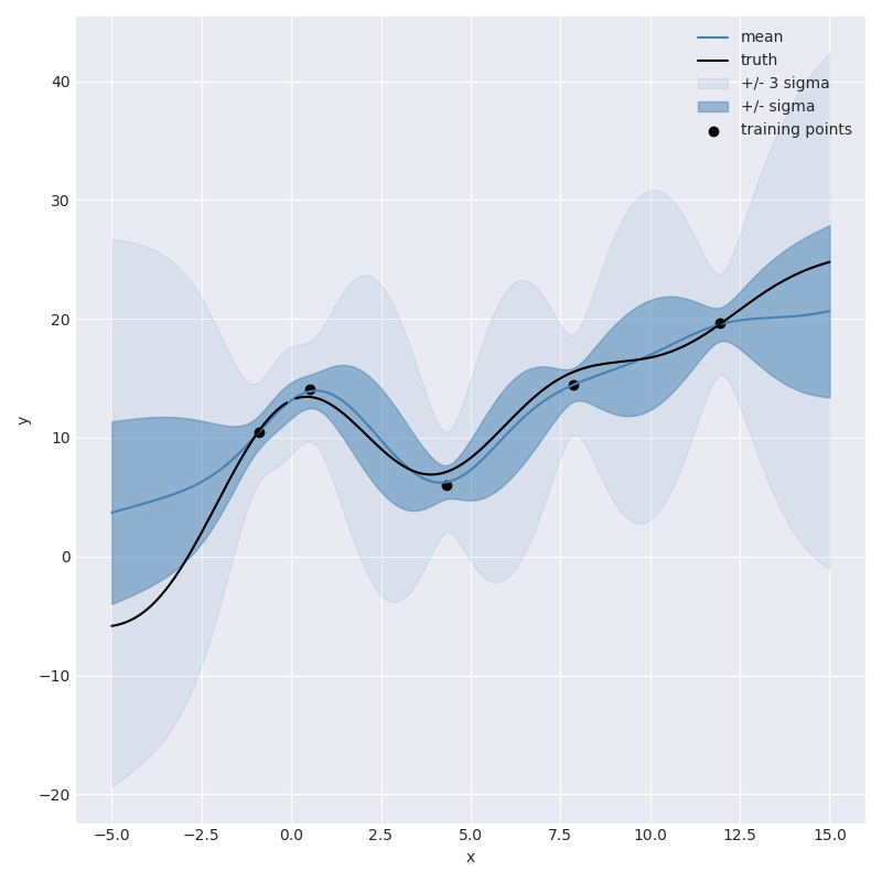
We built this model in albatross (see next section) and used synthetic data to give
us an idea of how the resulting model would perform:
From this plot we can see that the resulting model does a pretty good job of
capturing the non-linearity of the sinc function in the vicinity of training data,
including reasonable looking uncertainty estimates. However, you wouldn’t want to
use this model to extrapolate outside of the training domain since the predictions quickly
return to the prior prediction of 0.
To improve the model’s performance outside of the training domain we may want to introduce a systematic term to the model. For example instead of simply saying “the unknown function is non-linear but smooth” we may want to say “the unknown function is linear plus a non-linear smooth component.” We can do this by introducing a polynomial term into the covariance function.
More specifically we can define a covariance function which represents \(p(x) = a x + b\) by first placing priors on the values \(a\) and \(b\),
leading to the covariance function:
Where the first term captures the covariance between \(x\) and \(x'\) from the linear component and second term captures the covariance from the common offset.
Now we can assemble this into a new covariance function,
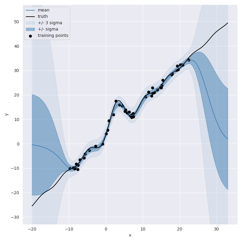
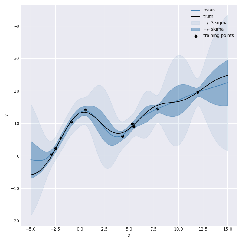
create a Gaussian process from it and plot the resulting predictions which look like:
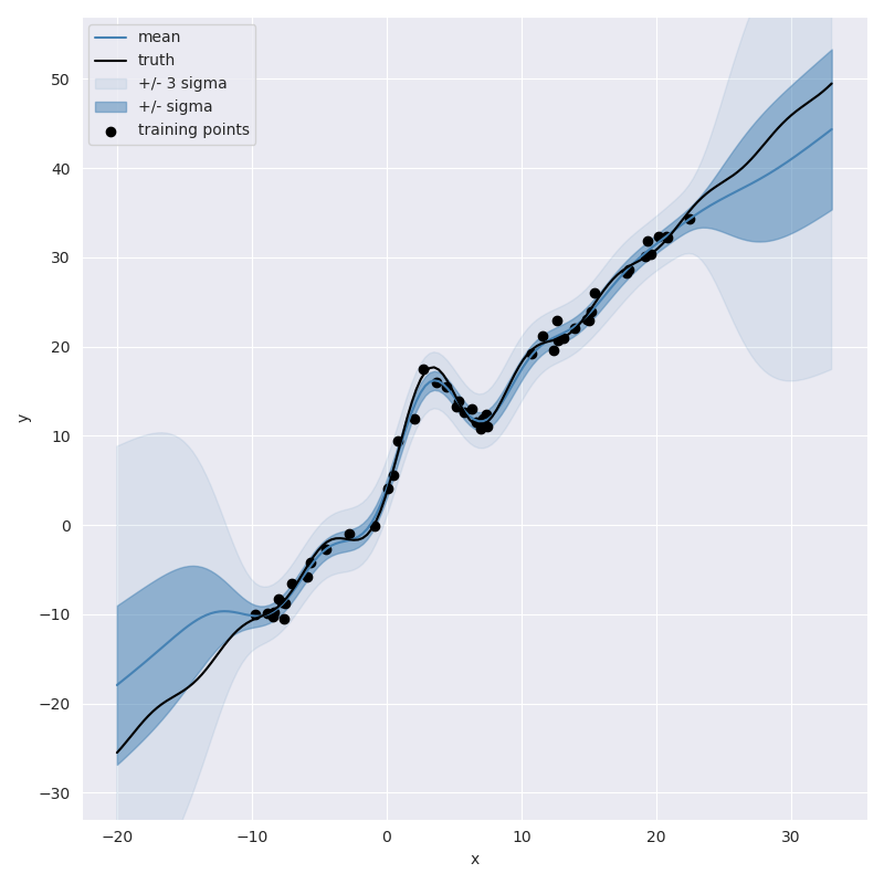
This plot shows that the model’s ability to extrapolate has been been significantly improved.
Implementation in albatross
One of the primary goals of albatross is to make iterating on model formulations
like we did in the examples above easy and flexible. All the components mentioned
earlier are already pre-defined. The creation of basic Gaussian
process which consists of a squared exponential term plus measurement noise, for example,
can be constructed as follows,
IndependentNoise<double> independent_noise;
SquaredExponential<EuclideanDistance> squared_exponential;
auto model = gp_from_covariance(sqrexp + independent_noise);
Similarly we can build a model which includes the linear (polynomial) term using,
IndependentNoise<double> independent_noise;
SquaredExponential<EuclideanDistance> squared_exponential;
Polynomial<1> linear;
auto model = gp_from_covariance(linear + sqrexp + independent_noise);
We can inspect the model and its parameters,
std::cout << covariance.pretty_string() << std::endl;
Which shows us,
((polynomal_1+independent_noise)+squared_exponential[euclidean_distance])
{
    {"sigma_independent_noise", 1},
    {"sigma_polynomial_0", 100},
    {"sigma_polynomial_1", 100},
    {"sigma_squared_exponential", 5.7},
    {"squared_exponential_length_scale", 3.5},
};
then condition the model on random observations, which we stored in data,
model.fit(data);
and make some gridded predictions,
const int k = 161;
const auto grid_xs = uniform_points_on_line(k, low - 2., high + 2.);
const auto predictions = model.predict(grid_xs);
Here are the resulting predictions when we have only two noisy observations,
2 Observations
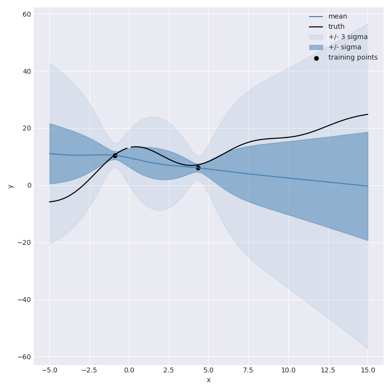
not great, but at least it knows it isn’t great. As we start to add more observations we can watch the model slowly get more confident,
5 Observations
10 Observations
30 Observations